6.6 Sequential Games
In this chapter, we’ll learn how to solve sequential games, which are strategic interactions where players make decisions in a specific order, with later players knowing the choices made by earlier players. We’ll visualize a sequential game using a game tree.
A sequential game consists of subgames, which begin with a decision node and include all nodes that follow it in the game tree. Every game tree has at least one subgame, because the game as a whole is always one of its subgames.
The equilibria of a sequential game is a subgame perfect equilibrium (SPE): an equilibrium that remains optimal in every subgame of a sequential game, meaning players’ strategies constitute best responses not only for the entire game but also in every smaller game that could be reached during play.
The key principle for finding SPE’s is that when analyzing sequential decisions, you should work backward using backward induction. The power of backward induction comes from systematically analyzing how current decisions interact with rational future responses. This provides a rigorous framework for strategic planning in sequential situations. An example will help to clarify:
Question 1: The Centipede Game
Two players alternate choosing to “take” or “pass”, starting with player A.
- If they “take”, the game ends and payoffs are distributed.
- If they “pass”, the pot grows bigger and the other player gets a turn.
Payoffs grow as follows:
- Stage 1: (2, 0) if take; continue if pass
- Stage 2: (0, 4) if take; continue if pass
- Stage 3: (6, 2) if take; continue if pass
- Stage 4: (4, 8) if take; end
Draw the game tree and solve for the subgame perfect equilibrium.
Suppose instead the payoffs for taking in stage 3 are (X, Y). Find the conditions on X and Y so that players will collaborate and grow the pot until stage 4.
Question 2: Jones Corporation
In a decision tree, squares represent decision nodes where the decision maker chooses between options, and circles to represent chance nodes where probability determines the outcome.
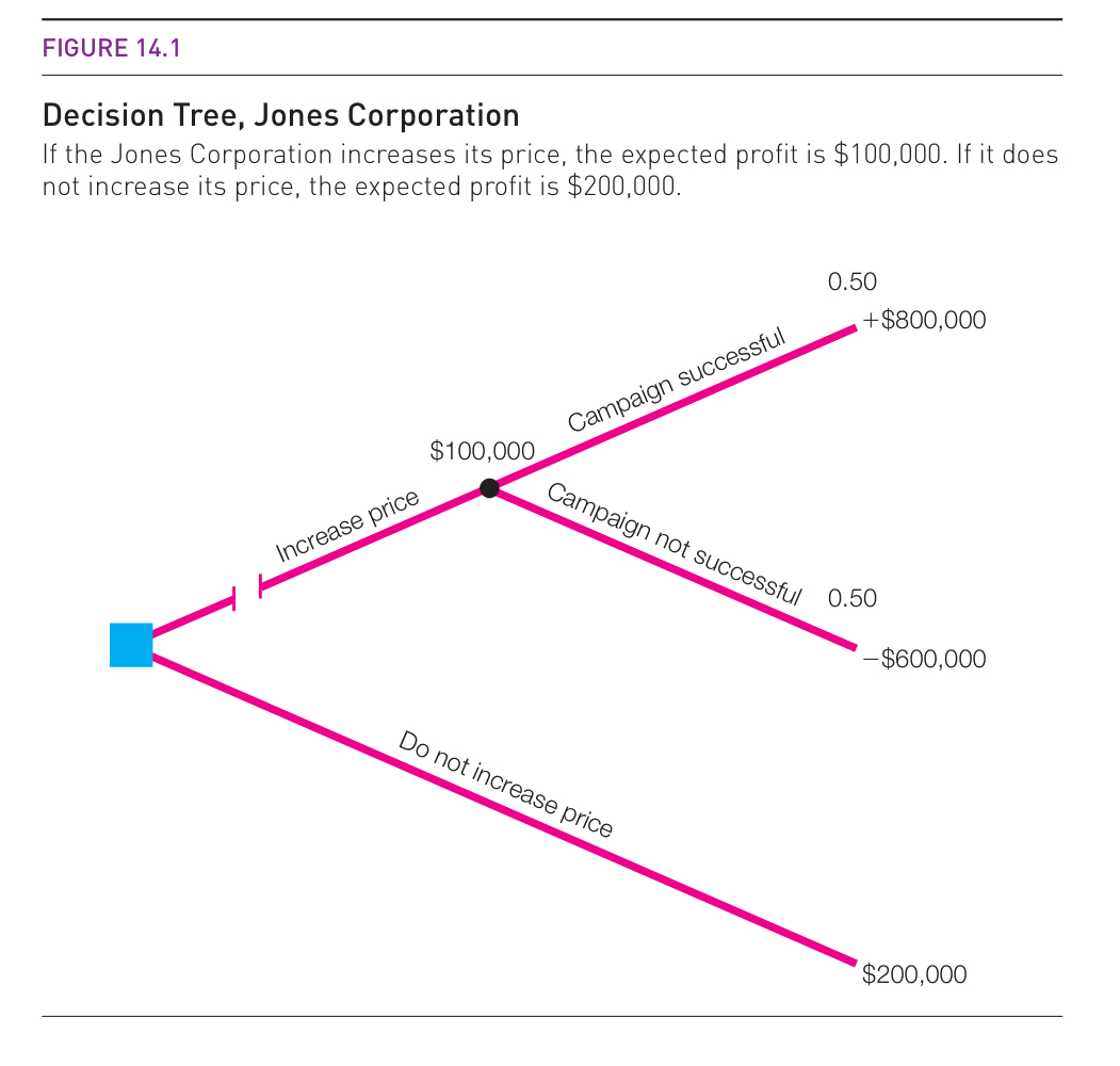
The Jones Corporation is considering a price increase (the blue square represents that choice). If they don’t increase the price (lower branch), they can continue on what they’re doing and earn an expected profit of $200K. If they increase the price, their fate is in the customer’s hands (black circle). Customers either accept the price increase, in which case they earn $800K in profit, or customers don’t accept it, and they lose $600K. If customers accept it and don’t accept it with equal probability, then the expected profit from increasing the price is \(0.5 \times 800\text{K} - 0.5 \times 600\text{K} = 100\text{K}\), which is why the upper branch is labelled $100K.
Assume the company is risk-neutral. The upper branch has an expected value of $100K and the lower one has an expected value of $200K: if the firm wants to maximize expected profit, it should choose the lower branch and not increase prices. This is represented by the two vertical lines through the upper branch to eliminate it.
If the campaign is successful with probability 0.6, should the company increase prices?
If the campaign is successful with probability 0.5, but the profit if the campaign is successful rises to $1M, should the company increase prices?
Question 3) Post-Graduation Decision Problem
Suppose Maria is graduating with an economics degree facing two options:
- Accept a consulting job offer ($50,000/year), or
- Take a year off to apply to MBA programs (outcome uncertain)
Draw a simple decision tree with these two branches. Represent Maria’s decision node with a square. In thousands, Maria’s expected value of accepting the consulting job offer right away is 50 + .9 (50) + .9^2 (50) + … . Calculate the value of this sum (this is your baseline for comparing her later options).
If Maria takes a year off to apply to MBA programs, there’s a 70% chance of acceptance to at least one program, and a 30% chance of rejection from all programs. If rejected, she can still take the consulting job after a year ($50,000/year). Update your decision tree and calculate the value of accepting the consulting job after a year (0 + .9(50) + .9^2 (50) + …).
If accepted, Maria takes 2 years to complete her MBA and she must choose between:
School 1: costs $30,000/year for 2 years. Then, she has a 50% chance of getting a marketing job ($100,000/year), and a 50% chance of getting a corporate strategy job ($120,000/year).
School 2: costs $80,000/year for 2 years. Then, she has a 20% chance of getting a job in finance ($180,000/year) and a 80% chance of getting a job at a nonprofit ($80,000/year)
Update your decision tree and calculate the total income for each branch (for example, if she chooses school 1 and gets the marketing job, she takes a year off to apply, spends 2 years in school, and then gets 100K/year after: 0 + .9(-30) + .9^2 (-30) + .9^(3) (100) + .9^4 (100) + …).
Assume Maria is risk-neutral and simply wants to maximize her discounted expected lifetime income. If accepted, should she choose school 1 or school 2? Draw a line through the school that is eliminated. Given that she can choose the school, should she apply to graduate school or not?
Question 4) Shortest Route to Downtown
Imagine a city map (shown in the figure below) where:
- The map connects residential areas to downtown parking lots
- Nodes represent intersections where drivers experience delays
- Lines represent streets connecting these intersections
- Numbers at each intersection show the delay time in minutes
The goal is to find the route from each residential area to downtown that minimizes the total time spent waiting at intersections. You might think to solve this by checking every possible path—all 150 of them—and picking the fastest one. However, this brute-force approach is very inefficient.
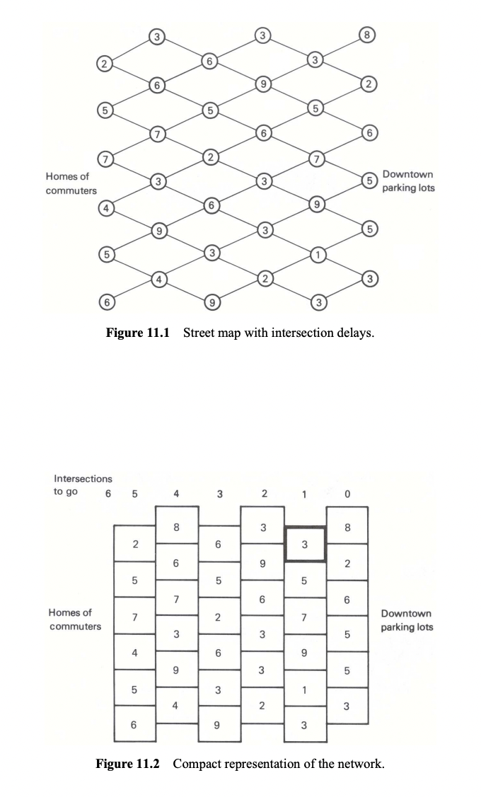
Instead use backward induction, by working from downtown (right side) to home (left side):
- Start with the final intersections (rightmost boxes):
- Here, there are no choices to make—you simply face whatever delay is shown
- Next, look at intersections one step from the end:
- Take the highlighted box in Figure 11.2 as an example
- At this intersection, you face:
- 3 minutes of delay at your current position
- Plus a choice: move up (8 minutes delay) or down (2 minutes delay)
- Best choice: Go down, for a total delay of 3 + 2 = 5 minutes
- Repeat this process for every intersection in that column:
- Calculate the total delay (current delay + best next move)
- Mark the best choice with an arrow (up or down)
- Write the minimum total delay