install.packages("haven")5.5 Nerlove (1963)
Returns to Scale in Electricity Supply
Part 1: Returns to Scale
Definition: Returns to Scale. Returns to scale describe how the output of a production process changes when all inputs are increased proportionally.
If output exactly doubles when inputs are doubled, the production process exhibits constant returns to scale. Mathematically: \(f(2x, 2y) = 2f(x, y)\).
If output increases by less than double, the production process has decreasing returns to scale. Mathematically: \(f(2x, 2y) < 2f(x, y)\).
If output more than doubles, the production process is said to have increasing returns to scale. Mathematically: \(f(2x, 2y) > 2f(x, y)\).`
Example
Suppose you have a pizza shop. What happens if you double everything - twice as much dough, twice as many ovens, twice as many workers, twice as much space? Will you make exactly twice as many pizzas? More than twice as many? Or less than twice as many?
It’s important to note that a firm can experience different types of returns to scale at different levels of production. For instance, a firm might experience increasing returns to scale when it’s small, constant returns to scale as it grows to a medium size, and then decreasing returns to scale if it becomes very large.
Constant returns to scale (CRS) is often considered a reasonable long-run expectation for many industries. This is because of the “replication argument.” The idea is that if a firm is operating at its most efficient scale, it should be able to simply replicate its entire operation to double its output. For instance, if a factory is operating efficiently, building an identical factory right next to it should double the output. However, while CRS might be a good theoretical baseline, real-world factors like limited resources, market size, or management complexities can lead to increasing or decreasing returns to scale in practice.
- Consider the Cobb-Douglas production function \(f(x_1, x_2) = x_1^{1/2} x_2^{1/2}\). Complete the proof to show this production function has constant returns to scale.
\[\begin{align} f(2 x_1, 2 x_2) &= (2 x_1)^{\_\_\_} (2 x_2)^{\_\_\_}\\ &= 2^{\_\_\_} x_1^{1/2} x_2^{1/2}\\ &= \_\_\_ f(x_1, x_2) \end{align}\]
- Consider the Cobb-Douglas production function \(f(x_1, x_2) = x_1 x_2\). Write a proof to show this production function has increasing returns to scale.
- The general Cobb-Douglas production function is given by \(f(x_1, x_2) = A x_1^a x_2^b\). Write a proof showing that the returns to scale depend on the magnitude of \(a + b\). Which values of \(a + b\) can be associated with which types of returns to scale?
Part 2: Data Project
Marc Nerlove’s 1963 study on the returns to scale in electricity supply is a foundational piece in the econometric analysis of cost structures in regulated industries. His work, “Returns to Scale in Electricity Supply,” published in Econometrica, found increasing returns to scale in the production of electricity, supporting the fact that electricity is a natural monopoly, and that electric companies should therefore be regulated as monopolies.
Nerlove’s work was part of a broader movement in applied econometrics that aimed to estimate production and cost functions rigorously. His approach was novel because it leveraged statistical methods to infer economies of scale directly from observed cost data.
Data
Run this code to download the original data set from Nerlove (1963).
library(tidyverse)

electric <- haven::read_dta("http://fmwww.bc.edu/ec-p/data/hayashi/nerlove63.dta")

electric
# A tibble: 145 × 5
totcost output plabor pfuel pkap
<dbl> <dbl> <dbl> <dbl> <dbl>
1 0.0820 2 2.09 17.9 183
2 0.661 3 2.05 35.1 174
3 0.990 4 2.05 35.1 171
4 0.315 4 1.83 32.2 166
5 0.197 5 2.12 28.6 233
6 0.0980 9 2.12 28.6 195
7 0.949 11 1.98 35.5 206
8 0.675 13 2.05 35.1 150
9 0.525 13 2.19 29.1 155
10 0.501 22 1.72 15 188
# ℹ 135 more rowsNerlove’s data is a cross-section on 145 firms in 44 states in the year 1955 for which data on all the relevant variables were available. Variables are:
totcost: total costs for the firmoutput: electricity output for the firmplabor: the wage rate (statewide average wages for utility workers)pfuel: price of fuel for the firmpkap: implied rental rate of capital equipment: derived from interest and depreciation charges available from the firm’s books
Data Inspection
Answer these questions using ggplot.
- How much does the wage rate differ across these 44 states?
- Do areas with higher wage rates have electric companies with higher costs? Answer this using ggplot or dplyr functions.
- How much does output differ across these electric companies?
- The rental rate of capital is the variable that is most imprecisely measured in the data. As the rental rate of capital increases, does the firm’s total costs increase?
Naive Approach
- Create a scatterplot with
log(totcost/output)on the y-axis andlog(output)on the x-axis. As output increases, it seems as though average costs decrease for firms.
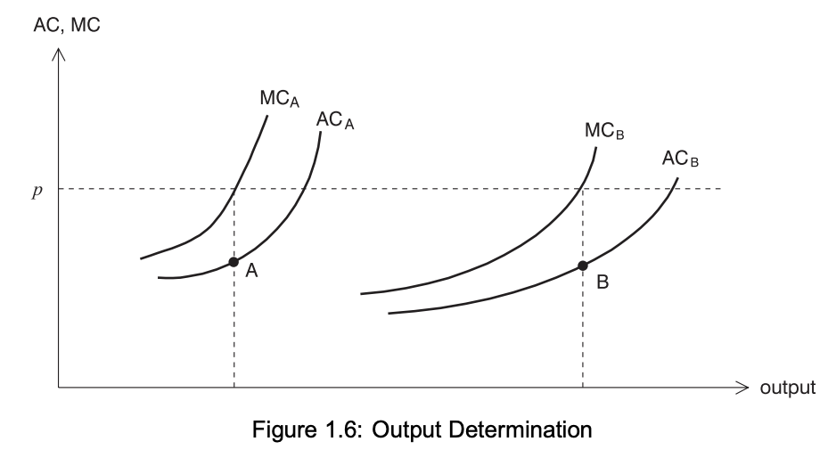
While it might seem intuitive, this is not enough evidence to say that firms have decreasing average costs (and thus increasing returns to scale). To understand why, consider the following along with the image below: each firm operates with its own unique cost structure, meaning their cost curves differ. Firms produce at the point where the market price (which represents their marginal benefit) intersects with their individual marginal cost curve. More efficient firms have lower marginal costs and, as a result, produce more output. This leads to lower average costs for firms that produce higher quantities. However, this does not imply that any firm’s average cost curve must be downward-sloping. The relationship between output and average costs can vary across firms without indicating increasing returns to scale.
Model
To derive a parameterized cost function, we start with the Cobb-Douglas production function:
\[Q_i = A_{i} x_{iL}^{\alpha_1} x_{iK}^{\alpha_2} x_{iF}^{\alpha_3}\]
- \(Q_i\) is firm i’s output
- \(A_i\) captures unobservable differences in production efficiency
- \(x_{iL}\) is labor input for firm i
- \(x_{iK}\) is capital input for firm i
- \(x_{iF}\) is fuel input for firm i
The sum \(r = \alpha_1 + \alpha_2 + \alpha_3\) is the degree of returns to scale.
Cost minimization gives us an equation for the total costs of the firm (see the bottom of this assignment for the derivation):
\[TC_i = r \cdot (A_i \alpha_1^{\alpha_1} \alpha_2^{\alpha_2} \alpha_3^{\alpha_3})^{-1/r} Q_i^{1/r} p_{i1}^{\alpha_1/r} p_{i2}^{\alpha_2/r} p_{i3}^{\alpha_3/r}\]
Taking logs:
\[\log(TC_i) = \mu_i + \frac{1}{r} \log(Q_i) + \frac{\alpha_1}{r} \log(p_{i1}) + \frac{\alpha_2}{r} \log(p_{i2}) + \frac{\alpha_3}{r} \log(p_{i3})\] where \(\mu_i = \log(r \cdot (A_i \alpha_1^{\alpha_1} \alpha_2^{\alpha_2} \alpha_3^{\alpha_3})^{-1/r})\).
- Estimate the linear model \(\log(TC) = \beta_0 + \beta_1 \log(Q) + \beta_2 \log(p_1) + \beta_3 \log(p_2) + \beta_4 \log(p_3)\) using lm().
- Interpretation: The parameter on log(output) tells us that the sum of the Cobb-Douglas exponents is \(\_\_\_\), which points to \(\_\_\_\) returns to scale. Electricity companies had decreasing average costs, and were therefore natural monopolies.
Answers:
Appendix: Cobb-Douglas Cost Minimization with 3 Inputs
\[\begin{align} &\text{Cobb-Douglas Production Function: }\\ &Q = A x_1^{\alpha_1} x_2^{\alpha_2} x_3^{\alpha_3}\\ &\text{Let r be the sum of the exponents: }\\ &r = \alpha_1 + \alpha_2 + \alpha_3\\ \\ &\text{Find the marginal products: }\\ &MP_1 = \alpha_1 A x_1^{\alpha_1 - 1} x_2^{\alpha_2} x_3^{\alpha_3}\\ &MP_2 = \alpha_2 A x_2^{\alpha_2 - 1} x_1^{\alpha_1} x_3^{\alpha_3}\\ &MP_3 = \alpha_3 A x_3^{\alpha_3 - 1} x_1^{\alpha_1} x_2^{\alpha_2}\\ \\ &\text{The tangency conditions are: }\\ &\frac{MP_1}{p_1} = \frac{MP_2}{p_2}\\ &\frac{MP_1}{p_1} = \frac{MP_3}{p_3}\\ \\ &\text{Equivalently: }\\ &\frac{MP_1}{MP_2} = \frac{p_1}{p_2}\\ &\frac{MP_1}{MP_3} = \frac{p_1}{p_3}\\ \\ &\text{Plug in for the marginal products: }\\ &\frac{\alpha_1 A x_1^{\alpha_1 - 1} x_2^{\alpha_2} x_3^{\alpha_3}}{\alpha_2 A x_2^{\alpha_2 - 1} x_1^{\alpha_1} x_3^{\alpha_3}} = \frac{p_1}{p_2}\\ &\frac{\alpha_1 A x_1^{\alpha_1 - 1} x_2^{\alpha_2} x_3^{\alpha_3}}{\alpha_3 A x_3^{\alpha_3 - 1} x_1^{\alpha_1} x_2^{\alpha_2}} = \frac{p_1}{p_3}\\ \\ &\text{Simplify and solve for x2 and x3: }\\ &x_2 = \frac{p_1}{p_2} \frac{\alpha_2}{\alpha_1} x_1\\ &x_3 = \frac{p_1}{p_3} \frac{\alpha_3}{\alpha_1} x_1\\ \\ &\text{Plug these into the production function: }\\ &Q = A x_1^{\alpha_1} x_2^{\alpha_2} x_3^{\alpha_3}\\ &Q = A x_1^{\alpha_1} \left(\frac{p_1}{p_2} \frac{\alpha_2}{\alpha_1} x_1 \right)^\alpha_2 \left(\frac{p_1}{p_3} \frac{\alpha_3}{\alpha_1} x_1 \right)^{\alpha_3}\\ \\ &\text{Solve for x1, the firm's demand for input 1: }\\ &\frac{1}{x_1^r} = \frac{A}{Q} \left(\frac{p_1}{p_2} \frac{\alpha_2}{\alpha_1}\right)^{\alpha_2} \left(\frac{p_1}{p_3} \frac{\alpha_3}{\alpha_1}\right)^{\alpha_3}\\ &x_1^r = \frac{Q}{A} \left(\frac{p_2}{p_1} \frac{\alpha_1}{\alpha_2} \right)^{\alpha_2} \left(\frac{p_3}{p_1} \frac{\alpha_1}{\alpha_3} \right)^{\alpha_3}\\ &x_1 = \left(\frac{Q}{A} \left(\frac{p_2}{p_1} \frac{\alpha_1}{\alpha_2} \right)^{\alpha_2} \left(\frac{p_3}{p_1} \frac{\alpha_1}{\alpha_3} \right)^{\alpha_3} \right)^{1/r}\\ &x_1 = \left(\frac{Q}{A}\right)^{1/r} \left(\frac{p_2^{\alpha_2} p_3^{\alpha_3}}{p_1^{\alpha_2 + \alpha_3}}\right)^{1/r} \left(\frac{\alpha_1^{\alpha_2 + \alpha_3}}{\alpha_2^{\alpha_2}\alpha_3^{\alpha_3}}\right)^{1/r} \\ \\ &\text{By symmetry, we also know demands for inputs 2 and 3: }\\ &x_2 = \left(\frac{Q}{A}\right)^{1/r} \left(\frac{p_1^{\alpha_1} p_3^{\alpha_3}}{p_2^{\alpha_1 + \alpha_3}}\right)^{1/r} \left(\frac{\alpha_2^{\alpha_1 + \alpha_3}}{\alpha_1^{\alpha_1}\alpha_3^{\alpha_3}}\right)^{1/r} \\ &x_3 = \left(\frac{Q}{A}\right)^{1/r} \left(\frac{p_1^{\alpha_1} p_2^{\alpha_2}}{p_3^{\alpha_1 + \alpha_2}}\right)^{1/r} \left(\frac{\alpha_3^{\alpha_1 + \alpha_2}}{\alpha_1^{\alpha_1}\alpha_2^{\alpha_2}}\right)^{1/r} \\ \\ &\text{Plug input demands into the total cost function: }\\ &TC = p_1 x_1 + p_2 x_2 + p_3 x_3\\ &TC = p_1 \left(\left(\frac{Q}{A}\right)^{1/r} \left(\frac{p_2^{\alpha_2} p_3^{\alpha_3}}{p_1^{\alpha_2 + \alpha_3}}\right)^{1/r} \left(\frac{\alpha_1^{\alpha_2 + \alpha_3}}{\alpha_2^{\alpha_2}\alpha_3^{\alpha_3}}\right)^{1/r} \right) + p_2 \left(\left(\frac{Q}{A}\right)^{1/r} \left(\frac{p_1^{\alpha_1} p_3^{\alpha_3}}{p_2^{\alpha_1 + \alpha_3}}\right)^{1/r} \left(\frac{\alpha_2^{\alpha_1 + \alpha_3}}{\alpha_1^{\alpha_1}\alpha_3^{\alpha_3}}\right)^{1/r} \right) + p_3 \left(\left(\frac{Q}{A}\right)^{1/r} \left(\frac{p_1^{\alpha_1} p_2^{\alpha_2}}{p_3^{\alpha_1 + \alpha_2}}\right)^{1/r} \left(\frac{\alpha_3^{\alpha_1 + \alpha_2}}{\alpha_1^{\alpha_1}\alpha_2^{\alpha_2}}\right)^{1/r} \right)\\ \\ &\text{Collect terms and simplify: }\\ &TC = \left(\frac{Q}{A}\right)^{1/r} \left(\frac{p_1 p_2^{\alpha_2/r} p_3^{\alpha_3/r}}{p_1^{(\alpha_2 + \alpha_3) / r}} \left(\frac{\alpha_1^{\alpha_2 + \alpha_3}}{\alpha_2^{\alpha_2} \alpha_3^{\alpha_3}} \right)^{1/r} + \frac{p_2 p_1^{\alpha_1/r} p_3^{\alpha_3/r}}{p_2^{(\alpha_1 + \alpha_3) / r}} \left(\frac{\alpha_2^{\alpha_1 + \alpha_3}}{\alpha_1^{\alpha_1} \alpha_3^{\alpha_3}} \right)^{1/r} + \frac{p_3 p_1^{\alpha_1/r} p_2^{\alpha_2/r}}{p_3^{(\alpha_1 + \alpha_2) / r}} \left(\frac{\alpha_3^{\alpha_1 + \alpha_2}}{\alpha_1^{\alpha_1} \alpha_2^{\alpha_2}} \right)^{1/r} \right) \\ &TC = \left(\frac{Q}{A}\right)^{1/r} \left(p_1^{\alpha_1/r} p_2^{\alpha_2/r} p_3^{\alpha_3/r}\right) \left( \left(\frac{\alpha_1^{(r - \alpha_1)/r}}{\alpha_2^{\alpha_2} \alpha_3^{\alpha_3}} \right)^{1/r} + \left(\frac{\alpha_2^{(r - \alpha_2)/r}}{\alpha_1^{\alpha_1} \alpha_3^{\alpha_3}} \right)^{1/r} + \left(\frac{\alpha_3^{(r - \alpha_3)/r}}{\alpha_1^{\alpha_1} \alpha_2^{\alpha_2}} \right)^{1/r} \right)\\ &TC = \left(\frac{Q}{A}\right)^{1/r} \left(p_1^{\alpha_1/r} p_2^{\alpha_2/r} p_3^{\alpha_3/r}\right) \left( \frac{\alpha_1^{(r - \alpha_1)/r} \alpha_1^{\alpha_1 / r} + \alpha_2^{(r - \alpha_2)/r} \alpha_2^{\alpha_2 / r} + \alpha_3^{(r - \alpha_3)/r} \alpha_3^{\alpha_3 / r}}{\alpha_1^{\alpha_1 / r} \alpha_2^{\alpha_2/r} \alpha_3^{\alpha_3/r}} \right)\\ &TC = \left(\frac{Q}{A}\right)^{1/r} \left(p_1^{\alpha_1/r} p_2^{\alpha_2/r} p_3^{\alpha_3/r}\right) \left( \frac{\alpha_1 + \alpha_2 + \alpha_3}{(\alpha_1^{\alpha_1} \alpha_2^{\alpha_2} \alpha_3^{\alpha_3})^{1/r}} \right)\\ &TC = \left(\frac{Q}{A}\right)^{1/r} \left(p_1^{\alpha_1} p_2^{\alpha_2} p_3^{\alpha_3}\right)^{1/r} \left( \frac{r}{(\alpha_1^{\alpha_1} \alpha_2^{\alpha_2} \alpha_3^{\alpha_3})^{1/r}} \right)\\ \end{align}\]