library(tidyverse)

# ggplot() +
#   stat_function(___) +
#   xlim(0, 50) +
#   ylim(0, 80) +
# labs(title = "Marginal Product of Fertilizer", x = "Fertilizer", y = "Marginal Product")5.2 Production Functions
A production function is a model for a producer that shows how inputs can be used to produce output.
For example, a (very) simple model of the production of wheat might be that the output of wheat is some function of the quantities of labor and fertilizer used: \(f(x_{labor}, x_{fertilizer})\).
A Cobb-Douglas production function has the form \(f(x_1, x_2) = A x_1^a x_2^b\) where \(a\) and \(b\) are non-negative and sum to 1. For example: \(f(x_{labor}, x_{fertilizer}) = 20 x_{labor}^{1/2} x_{fertilizer}^{1/2}\).
Part 1: Diminishing Marginal Product
Marginal benefits tend to decrease. We explored this in the previous assignment when I talked about my diminishing marginal enjoyment of beer. The first beer gives me a lot of enjoyment, but as I continue drinking, my enjoyment slips below the marginal cost of beer (the price or even the opportunity cost), and I stop buying beer.
In the same way, the first unit of fertilizer goes a long way toward increasing crop yield. But as you continue adding fertilizer, the marginal benefit decreases, and at some point, it slips below the marginal cost (price of a unit of fertilizer), at which point you should stop buying fertilizer.
- Show that the Cobb-Douglas production function for wheat \(f(x_{labor}, x_{fertilizer}) = 20 x_{labor}^{1/2} x_{fertilizer}^{1/2}\) has the property of diminishing marginal product for fertilizer. That is, take the partial derivative of \(f\) with respect to \(x_{fertilizer}\) and draw a plot with \(x_{fertilizer}\) on the x-axis and output \(f\) on the y-axis. You’ll need to set \(x_{labor}\) to be some constant: let’s say we employ 100 units of labor. As we increase the quantity of fertilizer, you should see that the marginal product (benefit) of fertilizer decreases.
Answer:
\[\begin{align} \frac{\partial f(x_{fertilizer}, x_{labor})}{\partial x_{fertilizer}} &= \\ \end{align}\]
Answer these questions by inspecting your plot from part A:
- Assuming we buy 100 units of labor, if the price (marginal cost) of a unit of fertilizer is $50, you should buy around ___ units because that’s where the marginal benefit is equal to the marginal cost.
- If the price (marginal cost) of a unit of fertilizer is $40, you should buy around ___ units.
- If the price (marginal cost) of a unit of fertilizer is $20, you should buy around ___ units.
- As the price of fertilizer falls, you should buy (more/less) fertilizer.
Answer:
Part 2: Isoquants
Isoquants are like indifference curves. They tell you all the sets of quantities of inputs that give you the same level of output. For example, to see the isoquant for 100 units of output, set \(f = 100\):
\[100 = 20 x_{fertilizer}^{1/2} x_{labor}^{1/2}\]
If we want to visualize this, solve for the variable you want to put on the y-axis:
\[\begin{align} x_{labor}^{1/2} &= \frac{100}{20 x_{fertilizer}^{1/2}}\\ x_{labor}^{1/2} &= \frac{5}{x_{fertilizer}^{1/2}}\\ x_{labor} &= \frac{25}{x_{fertilizer}} \end{align}\]
Then plug the right hand side into stat_function:
ggplot() +
  stat_function(fun = function(x) 25 / x, aes(color = "Output = 100")) +
  xlim(0, 30) +
  ylim(0, 30) +
  labs(title = "Isoquants", x = "Fertilizer", y = "Labor")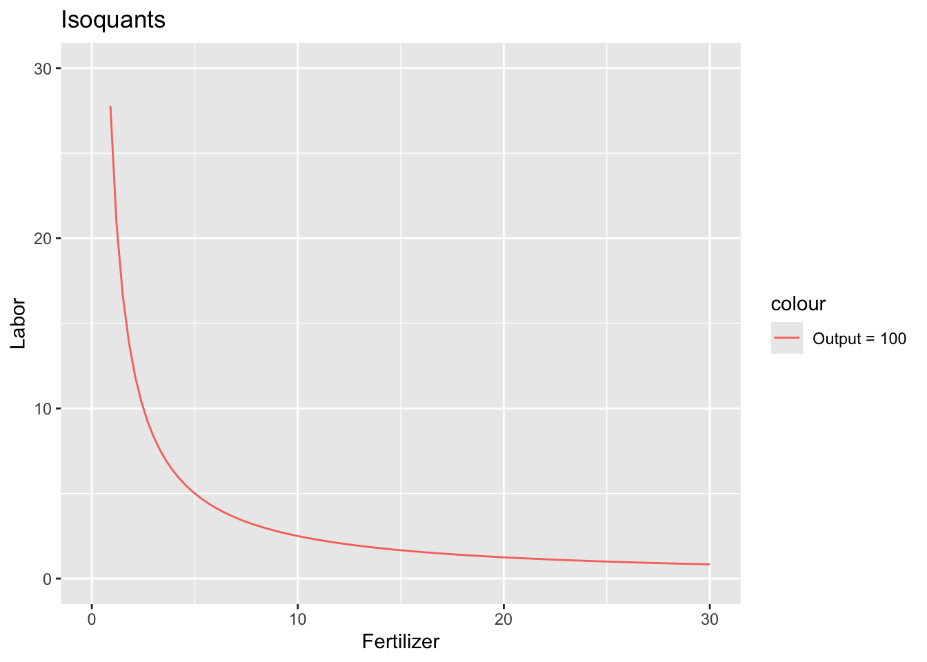
- Add two more isoquants to the plot: one representing all the input bundles required to produce 150 units of output, and another representing all the input bundles required to produce 200 units of output.
Answer:
# ggplot() +
#   stat_function(fun = function(x) 25 / x, aes(color = "Output = 100")) +
#   stat_function(___) +
#   stat_function(___) +
#   xlim(0, 30) +
#   ylim(0, 30) +
# labs(title = "Isoquants", x = "Fertilizer", y = "Labor")- Interpret: If you want to produce 100 units of output and you’re using 5 units of labor, you’d need ___ units of fertilizer. If you want to produce 100 units of output and you’re using 10 units of labor, you’d need ___ units of fertilizer. If you want to produce 100 units of output and you’re using 20 units of labor, you’d need ___ units of fertilizer.
Answer:
- Cobb-Douglas production functions show a preference for an even mixture of inputs instead of relying on one input too heavily. So if you can only afford a little labor, you need to buy much (less/more) fertilizer to compensate. And conversely, if you can only afford a little fertilizer, you need to hire much (less/more) labor to compensate.
Answer:
Part 3: Marginal Rate of Technical Substitution (MRTS)
Just like the MRS is the negative of the slope of the indifference curve, the MRTS is the negative of the slope of the isoquant. It’s the rise over the run: \(\frac{-dx_2}{dx_1}\). We’ll derive the formula by taking the total differential of the production function, setting \(df\) to be 0 (there is no change in output across the isoquant), and then solving for \(\frac{-dx_2}{dx_1}\):
\[\begin{align} df &= \frac{\partial f}{\partial x_1} dx_1 + \frac{\partial f}{\partial x_2} dx_2\\ 0 &= \frac{\partial f}{\partial x_1} dx_1 + \frac{\partial f}{\partial x_2} dx_2\\ - \frac{\partial f}{\partial x_2} dx_2 &= \frac{\partial f}{\partial x_1} dx_1\\ - \frac{dx_2}{dx_1} &= \frac{\partial f / \partial x_1}{\partial f / \partial x_2} \end{align}\]
- Find the MRTS of the production function \(f(x_{fertilizer}, x_{labor}) = 20 x_{fertilizer}^{1/2} x_{labor}^{1/2}\). Think about fertilizer as \(x_1\) and labor as \(x_2\).
Answer:
\[\begin{align} \frac{\partial f / \partial x_1}{\partial f / \partial x_2} &= \\ \end{align}\]
- Evaluate the MRTS at (1, 1). That is, if we are using 1 unit of fertilizer and 1 unit of labor, we could keep output the same by hiring a little more labor and a little less fertilizer at a rate of ___ units of labor to 1 unit of fertilizer.
Answer:
- Evaluate the MRTS at (100, 1). That is, if we are using 100 units of fertilizer and 1 unit of labor, we could keep output the same by hiring a little more labor and a little less fertilizer at a rate of ___ units of labor to 1 unit of fertilizer.
Answer:
- Evaluate the MRTS at (1, 100). That is, if we are using 1 unit of fertilizer and 100 units of labor, we could keep output the same by hiring a little more labor and a little less fertilizer at a rate of ___ units of labor to 1 unit of fertilizer.
Answer:
- Does the log trick work here? Repeat part A of this question, but take the natural log of the production function first. You should get the same answer for the MRTS, but the algebra is a little simpler.
Answer:
\[\begin{align} \log(f) &= \\ MRTS &= \\ \end{align}\]